THE GEOMETRIC DISTRIBUTION OF QUEUE LENGTH

UNDER A PREEMPTIVE-RESUME

LAST-COME-FIRST-SERVED

DISCIPLINE

APPROVED:

_________________________________

Robert Graham Landrum

1993

DEDICATION

This report is dedicated to my parents and the memory of Robert Todd Lapsley Liston and of Charles Adair Bledsoe. These have been the architects of my education.

THE GEOMETRIC DISTRIBUTION OF QUEUE LENGTH

UNDER A PREEMPTIVE-RESUME

LAST-COME-FIRST-SERVED

DISCIPLINE

ROBERT GRAHAM LANDRUM, B.S.

REPORT

Presented to the Faculty of the Graduate School of

The University of Texas at Austin

in Partial Fulfillment

of the Requirements

for the Degree of

MASTER OF ARTS

THE UNIVERSITY OF TEXAS AT AUSTIN

MAY 1993

Chapter One: Introduction and Explanation of Notation

A classic example of a queue is a group of patrons lined up to purchase concert tickets. The two parts of a queueing system consist of a serving facility (e.g. the ticket booth) and a queueing facility (e.g. the line of concert goers). In general the queueing facility may consist of a number of queues as in a supermarket's checkout lines; likewise the serving facility may have a number of servers. In this report models with one queue and mostly one server will be considered.

This kind of arrangement is often encountered; however there are other schemes that approximate other situations and have the advantage of easier calculation of relevant quantities. Once these calculations have been made, they may be transferred to a "normal" queue through a mathematical transformation. The difference in the models is in the queue discipline, which will be discussed presently.

The notation set out here is based on that of Leonard Kleinrock.[1] The nth customer, designated by C_n where n 0, enters the system at t_n . For calculation purposes t₀ = 0. The waiting time w_n is the time spent by C_n in the queue while x_n is the associated service time; furthermore the total system time for C_n is calculated as s_n = w_n + x_n. The difference t_n = t_n - t_n_-1 is the interarrival time between C_n_-1 and C_n. For most purposes the t_n's and the x_n's are considered to be independent. Now we may define

q_n = the number of customers in the system just after C_n departs.[2]

q'_n= the number of customers in the system just before C_n arrives.[3]

For each n the random variables t_n and x_n are the associated with the distribution functions A_n(t) and B_n(x) , and these values are the basis for the probabilistic nature of the setup. The related probability density functions (pdf's) are a_n(t) and b_n(x) respectively.

If a sequence of random variables converges (in probability) as n , then the corresponding limiting variable is denoted with a tilde: . Limiting distribution functions and their pdf's are written without a subscript e. g. A(t) and a(t).

The following variables may now be defined for the number of customers in the system:

p_k = [4]

d_k = Pr()

r_k = Pr() [5]

For and set . Define the utilization factor where m is the number of servers. Since it is the ratio of the average arrival rate to the average service rate for the system, 0 r 1 in order for an equilibrium state to occur; otherwise the servers will not be able to handle incoming customers fast enough.

The Laplace transform of the variable's pdf will be represented as

(1.1)

where H(y) = Pr(Y y) is a distribution function.[6] Similarly the z-transform – also called the generating function – for a discrete random variable is

. (1.2)

Here h_n = Pr(Y = n).[7]

In order to be classified succinctly, queues are designated with the form A/B/m where A and B stand for the distributions of the interarrival and service times respectively and m is the number of servers in the service facility. The distributions are denoted as follows:

G: General

M: (for Markov process) Exponential

E_r: r-stage Erlangian

H_R: R-stage hyperexponential

D: Deterministic

A M/H_R/2 queue, for example, has exponentially distributed interarrival times, services with an R-stage hyperexponential distribution, and employs two servers.[8]

How a customer progresses through the system is described by the queue discipline. The most common process is the first-come-first-served (FCFS) discipline where the next customer to be served is the one that has been in the queue the longest. This is like the concert goers buying tickets. An alternate scheme is called the last-come-first-served (LCFS) discipline. Here the next customer for service is the latest. (This is really a stack but will be called a queue.)

In this report the last-come-first-served queue discipline with preemptive resume will be explored usually for queues with one server. Its designation will be LCFS/I where the "I" stands for "interrupt." Upon the arrival of a customer into such a system, the customer in service leaves the server immediately and enters the queue; the new customer takes up the position with the server. If the customer with the server completes his service, he leaves the system, and the last customer to have entered the queue returns to the server. This will be the customer who was in service when the now departing one arrived.[9]

This report proceeds with a discussion of the intrinsic geometric nature of G/M/m queues. M/G/1 (LCFS/I) models are then explored through an intuitive interpretation of Beneš's inversion of the Polleczek-Khinchin Transform Equation. The last topic is G/G/1 (LCFS/I) systems with an expansion of the techniques used for the M/G/1 arrangement.

Chapter Two: The Queue Length in G/M/m Systems

In this chapter we will discuss the geometric distribution of queue length under an arbitrary queueing discipline, but the service time will be assumed to be exponentially distributed.

The mathematical basis for this analysis is the semi-Markov chain. Let X_n be a random variable that is paired with a time T_n where T_i < T_j for i < j. The sequence {X_n,T_n} is then a semi-Markov chain[10] if

(2.1)

Setting t to leaves

(2.2)

To be as general as possible, it will be assumed that there are m servers. The development follows that of Kleinrock.[11]

The random variables of the sequence q'_n} form a semi-Markov chain, and the relationship between successive pairs is easily established:

q'_n₊₁ = q'_n + 1 - v'_n₊₁ (n 0).(2.3)

Here v'_n₊₁ is the number of customers who finish being served and leave between the arrivals of C_n and C_n₊₁ . The transition probabilities are designated

p_ij = Pr(q'_n₊₁ = j | q'_n = i) (2.4)

or equivalently

p_ij = Pr(i + 1 - j customers leave during t_n₊₁ | q'_n = i). (2.5)

With the v'_n's being nonnegative, it follows immediately that

p_ij = 0 for j > i + 1. (2.6)

We will concentrate on the situation where i m. Since the service time is exponentially distributed,

. (2.7)

Now p_ij may be calculated for m j i + 1:

(2.8)

In this last equation the dependence on i and j is in the form i + 1 - j. Define n = i + 1 - j, and set

. (2.9)

b_n is the probability that n customers finish service in an interarrival time given that all m servers are occupied. Let E_k be the event that there are k customers in the system, and define

c_i(j) = the number of times that the state E_j is reached between successive visits to E_i.

s_k = E( c_k(k + 1) ) (k m – 1)

g = Pr( c_k_{+ 1} (j) = 0, j k) (k m – 1)

= Pr( c_k_{+ 1}(k) = 0)

N_k(t) = the number of times in (0, t) that an arriving customer finds the system in state E_k when the system starts at t = 0 with 0 customers.

Note that g is the same regardless of the value of k. In order to see this, suppose that a sequence of transitions between states results in c_k_{+ 1}(k) = 0 where k m – 1. Every such sequence can be matched one-to-one with a parallel sequence having the same relative transitions but starting with k + 2 customers in the initial system; furthermore this parallel sequence satisfies c_k_+ 2(k + 1) = 0 and has the same probability as the first. It is apparent that

Pr( c_k_+
1(k) = 0) = Pr( c_k_+
2(k + 1) = 0) k m – 1. (2.10)

The variable s_k may be thought of as the ratio of the times that the system is in state E_k_{+ 1} to the times it is in state E_k. It follows that

. (2.11)

If a(t) is the number of customers that have entered the system in (0, t), then

; (2.12)

consequently

. (2.13)

From Equation 2.1 it is apparent that if a system goes from a state E_k to E_k' (k < k'), it can only do so by rising through successive states; thus if a system in state E_k loses customers before a new customer can arrive, it must pass through E_k before reaching E_k_{+ 1}. In such a case c_k(k + 1) = 0. This indicates that

Pr(c_k(k + 1) > 0) = b₀. (2.14)

We may now calculate

Pr(c_k(k + 1) = n) = Pr(c_k(k + 1) > 0) [Pr(c_k_{+ 1}(k) = 0)]ⁿ^{– 1} Pr(c_k_{+ 1}(k) > 0)

= b₀gⁿ^–
1(1 – g), (2.15)

and

(2.16)

which reduces to

. (2.17)

Since the right side of this equation does not depend on k, we may drop the subscript: for k m – 1. (2.18)

From Equation 2.10

r_k_+
1 = sr_k k m – 1 (2.19)

r_k_+
1 = Ks^k k m – 1. (2.20)

Here is the geometric relation, but now we need to find K and s. With r_k being an equilibrium probability, the vector r = (r₀, r₁, r₂, r₃, . . .) is a solution of the equation r = rP where P = (p_ij). Explicitly, when all servers are known to be busy,

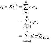(2.21)

Solving for s, we get

, (2.22)

which is equivalent to

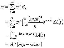(2.23)

By solving the last equation for a value in (0, 1), s may be determined. K then follows from the fact that .

Theorem: The length of the queue proper given that an arriving customer finds all servers busy is geometrically distributed.

Proof. Let Q be the event that an incoming customer must enter the queue; then

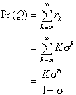(2.24)

and

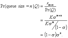(2.25)

This is the desired result.

Theorem: The number of customers in a G/M/1 system is geometrically distributed.

Proof:

(2.26)

which may be solved to yield

K = 1 – s. (2.27)

The intended result r_k = (1 – s)s^keasily follows.

The geometric nature of these systems comes from the circumstance of b₀ , g, and thus s_k being independent of k. As was shown earlier, g was developed without appealing to the underlying probability distributions. On the other hand, the independence of b₀ from k was evidenced in Equation 2.8 which was derived from the Poisson distribution of departing customers: the exponential service times are central to this argument although there is no need for a special queueing discipline.

Chapter Three: M/G/1 (LCFS/I) Systems

Although the material in this chapter is less general than that in the next chapter, it provides an insight into what is actually occurring with the LCFS/I discipline.

The value of the exponential distribution is that it is memoryless – that is Pr(t > s+t |t > s) = Pr(t > t).[12] In the G/M/m case this meant that only the time between arrivals was needed to calculate the number of departures for that period: the time between the last departure and first arrival could be "forgotten." For M/G/1 systems the situation is reversed: since the arrivals are exponentially distributed, the semi-Markov chain is established on the sequence {q_n} of departure times.

3.1. Beneš's Inversion of the Pollaczek-Khinchin Formula for Waiting Time

For this section we need three distribution functions:

Q(t) = Pr()

S(t) = Pr()

W(t) = Pr()

Q^#(z) can be obtained from the Pollaczek-Khinchin Transform Equation:

.[13] (3.1)

Another form of this generating function may be calculated using the FCFS discipline. In this case all the q_n customers in the system when C_n leaves arrive during C_n's system time. Since interarrival times are exponentially distributed, q_n has a Poisson distribution:

. (3.2)

Integrating with respect to s and taking the limit as , we get

. (3.3)

Now we calculate[14]

(3.4)

Setting s = l - lz and combining Equations 3.1 and 3.4, we get

. (3.5)

The equation leads to

S*(s) = W*(s)B*(s), (3.6)

which may be used to get

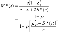(3.7)

The residual life distribution for the service time is

, (3.8)

and

;[15] (3.9)

thus

(3.10)

If is the k-fold convolution of , set

; (3.11)

then

.[16] (3.12)

3.2. An Attempt to Explain the Formula Directly with a FCFS Discipline

From the results in Chapter Two one may calculate that r_k = (1 – r)r^k for M/M/1 queues; also since in this case, is the probability that the sum of k service times is less than t. This suggests that the following interpretation of Equation 3.12 is plausible:

. (3.13)

Now consider a M/D/1 (FCFS) setup where , a constant. In this case

. (3.14)

From the Pollaczek-Khinchin Transform Equation,

. (3.15)

Expanding this in a Taylor series, one obtains the d_k's as the respective coefficients of the z^k's. Since changes by integer increments, r_k = d_k and the following table may be constructed[17]:

(3.16)

Clearly this is not the geometric distribution intimated in Equation 3.12; furthermore and B(t) do not generally coincide. Equation 3.12 was useful for calculating purposes but did not seem to have an intuitive explanation.

3.3. Cooper and Niu's Explanation using LCFS/I

Equation 3.13, with a new interpretation for , was shown to be the correct explanation by Robert Cooper and Shun-Chen Niu in their 1986 article.[18] The core of their calculations is in the following theorem.

Theorem: The number of customers in a M/G/1 (LCFS/I) queue is geometrically distributed with r_k = (1 – r)r^k.

Proof. Define

= the residual time for the service after being interrupted. It has distribution function .

A queueing system can only reach a state E_k directly either by beginning in E_k_–
1 and having a customer arrive or by being in E_k_{+ 1} and losing a customer. In the latter case when a last-come-first-served arrangement is used, the service time of the customer then entering service is actually a continuation of the service period interrupted by the now departing customer: the new service interval is a residual one. We may now determine that

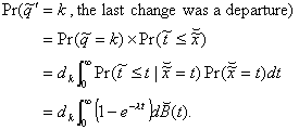(3.17)

Note that d_k is used as opposed to d_k₊₁ because this random variable refers to the number of customers after the departure from the k+1 state. A similar calculation yields

(3.18)

It now follows that

(3.19)

Since a departing customer leaves the system in the same exact condition as when he arrived, d_k = r_k; thus

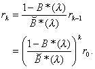(3.20)

Knowing that r₀ = 1 –r and using the normalization condition, we find that

(3.21)

and

r_k = (1 – r)r^k. (3.22)

Equation 3.21 may be rewritten as

, (3.23)

which being essentially Equation 3.9 –l is after all an arbitrary positive number – gives that .[19]

In order to understand , one needs to define the function U(t) which gives the work time that remains to be done by the server at time t. If

(3.24)

where

(3.25)

is the heavy side step function, then

. (3.26)

U(t) is a nonnegative function that jumps up x_n in height at each t_n. From these points it descends with a slope of –1 until another jump occurs or until U(t) = 0. In the latter case it remains flat up to the point where a new customer arrives. The positive portions of the function represent the system's busy periods. The complementary idle periods are the segments where U(t) = 0.[20]

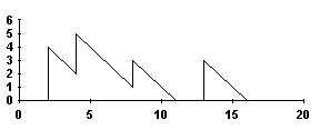U(t)

Figure 3.1

The form of U(t) does not depend on how the customers are served; however in the FCFS case the remaining work time just before a customer arrives is that customer's waiting time: . One may interpret as the equilibrium remnant work time just before a customer arrives. It is now straightforward to show that in a LCFS/I system, and Equation 3.13 then follows. Beneš's inversion of the Pollaczek-Khinchin Transform Equation, which was developed from a FCFS discipline, is more closely related to a LCFS/I discipline.

Chapter Four: G/G/1 (LCFS/I) Systems

Without the exponential distribution analysis of queues becomes more difficult. Semi-Markov processes can not be used in the same way as they were used for the G/M/m model: besides the interarrival times the times between a preceding departure and an arrival become important. The study of G/G/1 queues centers on ascending ladder points.

4.1. Preliminaries

Set

, (4.1)

where q(t) is again the step function.

R(t) is a function with a –1 slope that jumps up x_n at each t_n: it is similar to U(t) except that it descends below zero.[21] The values just before the jumps will be designated , and the difference in successive peaks will be u_n = U_n₊₁ – U_n for n 0. It can be deduced from Equation 4.1 that u_n = x_n – t_n₊₁.[22]

Define a new sequence n_k starting with n₁ set such that is the first peak to exceed U₀ = 0. Assign n_k_{+ 1} so that is the first peak after with . is the set of ascending ladder indices.

In a stable queue r < 1 or 1/m - 1/l < 0. This equation implies that E[u_n] < 0, and consequently . The result is that there can only be a finite number of ascending ladder indices. Set K equal to this number, and designate s = Pr(K 1).

Suppose that R(t) reaches . Since the u_n's are independent identically distributed random variables, the probability that there is a point of R(t) that exceeds is the same as the probability that R(t) rises above 0; therefore

Pr(K k + 1) = Pr(K 1 ) Pr(K k) = sPr(K k). (4.2)

This leads to

Pr(K = k) = (1 – s)s^k. (4.3)

For K = k, set

, (4.4)

and

. (4.5)

The 's are also independent identically distributed random variables. They represent the idle times in the dual queue[23] where the service and interarrival distributions are swapped. Let F(x) = Pr( x) and designate its nth convolution with itself with

(4.6)

For the u_n's the common distribution function will be

. (4.7)

It will be important to specify notation for the customers currently in the queue. If 0, then set equal to the remaining service time of the ith customer still in the queue. The index i ranges from i = 1 for the customer that has been there longest to i = k for the most recent one.[24]

4.2. A Theorem by D. Fakinos

Theorem: In a G/G/1 (LCFS/I) system,

(4.8)

where s and F(t) are defined in the previous section.[25]

Proof. Consider what is necessary for a stationary distribution:

(4.9)

For k = 0 and n > 0,

. (4.10)

In the limit as n this leads to

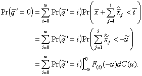(4.11)

For k > 0 and n > 0,

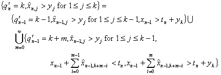(4.12)

which, in the limit, becomes

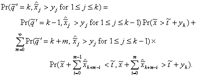(4.13)

From the preliminary material it may be deduced that

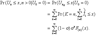(4.14)

which transforms into

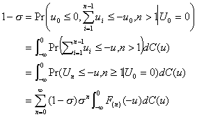(4.15)

The event is really the event that for K = k, and given that U₀ = 0. This may be restated as

(4.16)

This leads to

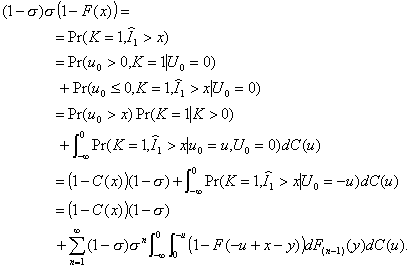(4.17)

If the theorem is correct, Equation 4.8 must satisfy Equations 4.11 and 4.13. In this light Equation 4.13 becomes

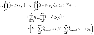(4.18)

(4.19)

which agrees with Equation 4.17. Equation 4.11 agrees with Equation 4.15 in the same way. It follows that Equation 4.8 is a stationary distribution for the system and holds true in the limit.

To show that this solution is unique, note that since r < 1, the state for q' = 0 is non-null persistent. The probability r₀ = 1 - s is independent of the initial state; and when the queue reaches that state the succeeding condition of the system is independent of preceding conditions. The queue is ergodic and can only assume the character of the given solution.

4.3 A Result Based on Cooper and Niu's Argument

Usually the semi-Markov process is established solely on the set of arrival instances or solely on the set of departure instances. Since arrivals and departures affect the server for a LCFS/I queue, a semi-Markov process can be set up incorporating both types of events. In this light let

(4.20)

In this type of system a customer need only "see" the customers who enter the queue after him. In fact he need only be concerned with the customers who immediately interrupt his service and consequently "block" his "view" until they have finished all their service time. This suggests that changes in state do not depend on the actual queue length but may be described by the following probabilities:

a_a = Pr(arrival | the last event was an arrival)

a_d = Pr(arrival | the last event was a departure)

d_a = Pr(departure | the last event was an arrival) (4.21)

d_d = Pr(departure | the last event was a departure)

These are further described by

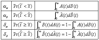
Table 4.1

Here is the residual time of an interrupted interarrival period:

[26] (4.22)

Consider the value of at an arrival:

. (4.23)

Using the same methods of Section 3.3, one gets

(4.24)

and

(4.25)

likewise

(4.26)

With this,

(4.27)

(4.28)

Comparing this with Equation 4.8, one sees that

(4.29)

This produces a method for calculating a constant that was previously defined abstractly.

[1]Leonard Kleinrock, Queueing Systems, I (New York: Wiley-Interscience, 1975), pp. 10-18, 396-399.

[9]D. Fakinos, "The G/G/1 Queuing System with a Particular Queue Discipline," Journal of the Royal Statistical Society B, 43 (1981) 190.

[10]U. Narayan Bhat, Elements of Applied Stochastic Processes, 2nd ed. (New York: John Wiley & Sons, 1984), p. 290.

[18]Robert B. Cooper and Shun-Chen Niu, "Beneš's Formula for M/G/1-FIFO 'Explained' by Preemptive-Resume LIFO," Journal of Applied Probability, 23 (1986) 550-554.

[25]D. Fakinos, "The G/G/1 Queueing System with a Particular Queue Discipline," Journal of the Royal Statistical Society B, 43 (1981), pp. 190-196.

Bibliography

Bhat, U. Narayan. Elements of Applied
Stochastic Processes, 2nd ed. New York: John Wiley & Sons, 1984.
Cooper, Robert B., and Niu, Shun-Chen. "Beneš's Formula for M/G/1-FIFO
'Explained' by Preemptive-Resume LIFO." Journal of Applied Probability, 23 (1986) 550-554.
Fakinos, D. "The G/G/1 Queueing System with a Particular Queue
Discipline." Journal of the Royal
Statistical Society, B 43 (1981)
190-196.
Kleinrock, Leonard. Queueing Systems, Vol. 1 New York:
Wiley-Interscience, 1975.
VITA
Robert Graham Landrum was born in Bristol, Tennessee, on
August 9, 1966, the son of Mary Fisher Landrum, M.A. and Graham Gordon Landrum,
Ph.D. After attending Tennessee High School, Bristol, Tennessee, he entered
King College, also of the same town, in 1983. He attended Purdue University for
the summer of 1985, and during the summer of 1986, he pursued research at
Lowell Observatory. In May of 1987 he graduated from King College with the
degree of Bachelor of Science. In September, 1987, he entered The Graduate
School of The University of Texas at Austin.
Permanent Address: 2115 Edgemont Avenue
Bristol,
Tennessee
37620-4745
This report
was typed by the author.
Leonard Kleinrock, Queueing
Systems, I (New York: Wiley-Interscience, 1975), pp. 10-18, 396-399.
D. Fakinos, "The G/G/1 Queuing System with a
Particular Queue Discipline," Journal
of the Royal Statistical Society B, 43 (1981) 190.
U. Narayan Bhat, Elements
of Applied Stochastic Processes, 2nd ed.
(New York: John Wiley & Sons, 1984), p. 290.
Robert B. Cooper and Shun-Chen Niu, "Beneš's
Formula for M/G/1-FIFO 'Explained' by Preemptive-Resume LIFO," Journal of Applied Probability, 23
(1986) 550-554.
Cooper and Niu, pp. 552-554.
D. Fakinos, "The G/G/1 Queueing System with a
of the Royal Statistical Society B, 43 (1981), pp. 190-196.
![]() . Limiting distribution functions and their pdf's are written
without a subscript e. g. A(t) and a(t).
. Limiting distribution functions and their pdf's are written
without a subscript e. g. A(t) and a(t).![]() [4]
[4]![]() )
)![]() ) [5]
) [5]![]() and
and ![]() set
set ![]() . Define the utilization factor
. Define the utilization factor![]() where m is the
number of servers. Since it is the ratio of the average arrival rate to the
average service rate for the system, 0 r 1 in order for an equilibrium state to occur;
otherwise the servers will not be able to handle incoming customers fast
enough.
where m is the